DL: StarDist and Cellpose#
StarDist and Cellpose are the two most popular deep neural network to perform object detection and segmentation. Let’s try them out with bioimageloader.
NOTE I am not trying to make a statement through this example that one model is better than the other. What I want to demonstrate here is that both models are fabulous and may or may not perform well depending on datasets.
NOTE This notebook requires around 4GB of GPU memory if you choose to use a GPU. If your GPU cannot cope with it then try running each model separately after reinitializaing the kernel.
Install dependencies and Imports#
notes about ``tensorflow``
We need stardist, which can be easily installed through pip (through https://pypi.org/), but what’s more important is to install tensorflow pkg. If you would like to use GPU, please find a guide in “Miscellaneous” ->“TensorFlow installation” in bioimageloader documentation.
Additionally we install matplotlib and seaborn for plotting and pandas, showing process using tqdm.
[1]:
# Choose a GPU if you have multiple ones
# tensorflow tries to use all available GPU on machine by default
# Ignore this part if you are going to use CPU
%env CUDA_VISIBLE_DEVICES=0
env: CUDA_VISIBLE_DEVICES=0
[2]:
# disable tf warning. Not a good idea in general
# I am hiding warnings for the sake of desmonstrating this notebook
%env TF_CPP_MIN_LOG_LEVEL=3
# TF assigns all available GPU memory to its processes by default
# Come on TF seriously, we don't like this behavior and not everyone
# sets up a virtual machine with a limited GPU memory setting.
# https://github.com/tensorflow/tensorflow/issues/25138
%env TF_FORCE_GPU_ALLOW_GROWTH='true'
env: TF_CPP_MIN_LOG_LEVEL=3
env: TF_FORCE_GPU_ALLOW_GROWTH='true'
[3]:
# #--- StarDist and Tensorflow ---# #
# !pip install csbdeep  # contains tools for restoration of fluorescence microcopy images (Content-aware Image Restoration, CARE). It uses Keras and Tensorflow.
# !pip install stardist # contains tools to operate STARDIST.
# !pip install gputools # improves STARDIST performances (optional)
# #--- Cellpose and PyTorch ---# #
# !pip install cellpose
# #--- etc ---# #
# !pip install matplotlib seaborn pandas tqdm
[4]:
import pandas as pd
import matplotlib.pyplot as plt
import seaborn as sns

# StarDist and TensorFlow
import tensorflow as tf
from stardist.models import StarDist2D
from stardist.data import test_image_nuclei_2d
from stardist.plot import render_label
from csbdeep.utils import normalize
from stardist.matching import matching

# Cellpose and PyTorch
import torch
from cellpose import models as cellpose_models

# bioimageloader
import albumentations as A
from bioimageloader import Config, BatchDataloader
from bioimageloader.transforms import SqueezeGrayImageHWC, HWCToCHW
from bioimageloader.utils import random_label_cmap

from tqdm.notebook import tqdm

plt.rcParams['font.size'] = 9
plt.rcParams['image.interpolation'] = 'none'
cmap = random_label_cmap()
[5]:
# setting 'TF_FORCE_GPU_ALLOW_GROWTH' does not actually limit
# gpu memory, it allows to grow. we have to manually limit memory usage
if gpus := tf.config.list_physical_devices('GPU'):
    for gpu in gpus:
        try:
            vdc = tf.config.experimental.VirtualDeviceConfiguration(
                memory_limit=2000
            )
            tf.config.experimental.set_virtual_device_configuration(
                gpu, [vdc]
            )
        except RuntimeError as e:
            print(e)
# see what devices you have (set)
print(tf.config.list_physical_devices())
[PhysicalDevice(name='/physical_device:CPU:0', device_type='CPU'), PhysicalDevice(name='/physical_device:GPU:0', device_type='GPU')]
StarDist#
Test StarDist#
Let’s check if everything works
I followed this guide on github page (https://github.com/stardist/stardist#pretrained-models-for-2d)
[6]:
model = StarDist2D.from_pretrained('2D_versatile_fluo')
# print info (I always like to know the details)
model.config.__dict__
Found model '2D_versatile_fluo' for 'StarDist2D'.
Loading network weights from 'weights_best.h5'.
Loading thresholds from 'thresholds.json'.
Using default values: prob_thresh=0.479071, nms_thresh=0.3.
[6]:
{'n_dim': 2,
 'axes': 'YXC',
 'n_channel_in': 1,
 'n_channel_out': 33,
 'train_checkpoint': 'weights_best.h5',
 'train_checkpoint_last': 'weights_last.h5',
 'train_checkpoint_epoch': 'weights_now.h5',
 'n_rays': 32,
 'grid': (2, 2),
 'backbone': 'unet',
 'n_classes': None,
 'unet_n_depth': 3,
 'unet_kernel_size': [3, 3],
 'unet_n_filter_base': 32,
 'unet_n_conv_per_depth': 2,
 'unet_pool': [2, 2],
 'unet_activation': 'relu',
 'unet_last_activation': 'relu',
 'unet_batch_norm': False,
 'unet_dropout': 0.0,
 'unet_prefix': '',
 'net_conv_after_unet': 128,
 'net_input_shape': [None, None, 1],
 'net_mask_shape': [None, None, 1],
 'train_shape_completion': False,
 'train_completion_crop': 32,
 'train_patch_size': [256, 256],
 'train_background_reg': 0.0001,
 'train_foreground_only': 0.9,
 'train_sample_cache': True,
 'train_dist_loss': 'mae',
 'train_loss_weights': [1, 0.2],
 'train_class_weights': (1, 1),
 'train_epochs': 800,
 'train_steps_per_epoch': 400,
 'train_learning_rate': 0.0003,
 'train_batch_size': 8,
 'train_n_val_patches': None,
 'train_tensorboard': True,
 'train_reduce_lr': {'factor': 0.5, 'patience': 80, 'min_delta': 0},
 'use_gpu': False}
[7]:
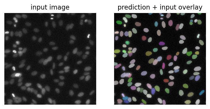
img = test_image_nuclei_2d()

labels, _ = model.predict_instances(normalize(img))

plt.figure(dpi=150)
plt.subplot(1,2,1)
plt.imshow(img, cmap="gray")
plt.axis("off")
plt.title("input image")

plt.subplot(1,2,2)
plt.imshow(render_label(labels, img=img))
plt.axis("off")
plt.title("prediction + input overlay")
[7]:
Text(0.5, 1.0, 'prediction + input overlay')
Test StarDist with bioimageloader#
Once we have a working StarDist, now it is time to have some fun with bioimageloader!
We will resize images to manageable size (256, 256) and squeeze channels.
Small but lengthy notes
bioimageloader provides a few custom transforms compatible with albumentations library. SqueezeGrayImageHWC is one of them. We already converted images to grayscale, but by default bioimageloader keeps its dimension to 3 channels because most computer vision models expect RGB channels (read more about assumptions and decisions bioimageloader made in the documentation). Long story short, SqueezeGrayImageHWC picks only one channel out of the same 3 channels.
[8]:
# give a path to dataset and set grayscale=True
cfg = {
    'DSB2018': {
        'root_dir': '../Data/DSB2018',
        'grayscale': True
    },
}
config = Config.from_dict(cfg)

transforms = A.Compose([
    A.Resize(256, 256),
    SqueezeGrayImageHWC()  # from (3, h, w) to (1, h, w)
])

datasets = config.load_datasets(transforms=transforms)
for dset in datasets:
    print(f'{dset.acronym:10s}: {len(dset):10d}')
DSB2018 : 670
Use bioimageloader.BatchDataloader to load data in batch
[9]:
# Feel free to adjust
BATCH_SIZE = 4
NUM_WORKERS = 2

dsb2018 = datasets[0]
loader = BatchDataloader(dsb2018,
                         batch_size=BATCH_SIZE,
                         num_workers=NUM_WORKERS)
iter_loader = iter(loader)
[10]:
data = next(iter_loader)
input_image = data['image']
# will have shape (BATCH_SIZE, 256, 256)
predictions = []
for i in range(BATCH_SIZE):
input_image_i = normalize(input_image[i])
pred, _ = model.predict_instances(input_image_i)
predictions.append(pred)
with plt.rc_context({'image.interpolation': 'none'}):
fig, ax = plt.subplots(nrows=BATCH_SIZE, ncols=2,
figsize=[8, 4*BATCH_SIZE],
dpi=150)
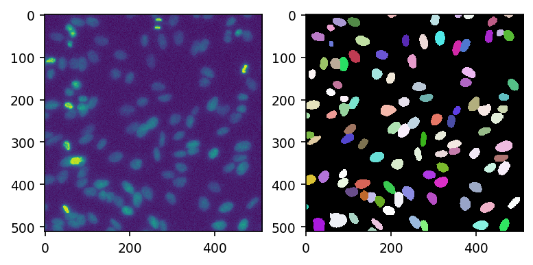
for i, (img, pred) in enumerate(zip(input_image, predictions)):
ax[i, 0].imshow(img)
ax[i, 0].set_title('image')
ax[i, 1].imshow(pred, cmap=cmap)
ax[i, 1].set_title('prediction')
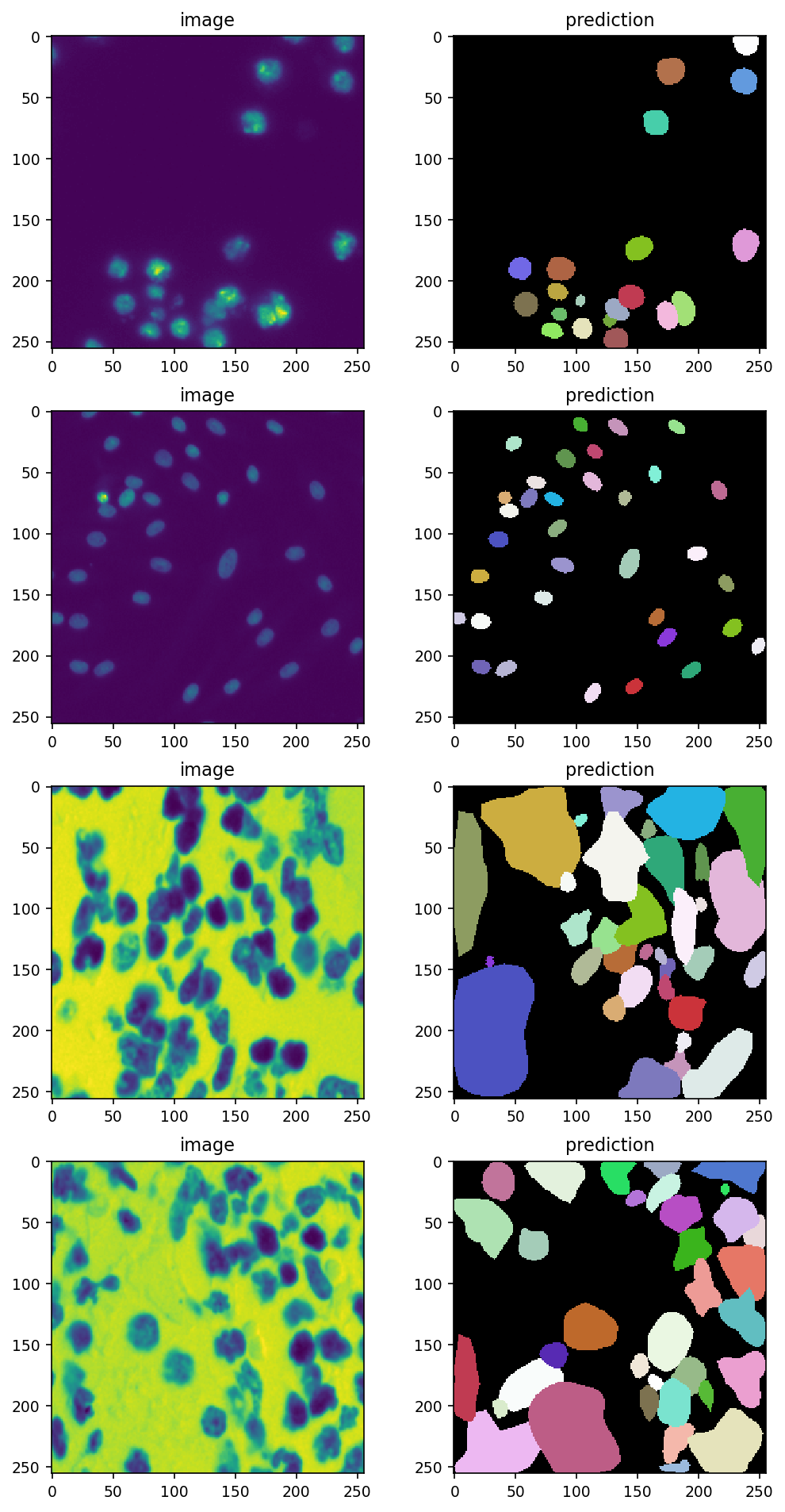
Notice how easy it was to load data and run StarDist on them with bioimageloader? Let’s have some more fun.
*The thrid and the forth one had better be inverted. Anyway let’s keep going on.
Evaluation#
Using bioimageloader, we can easily iterate through all images of DSB2018 and get metric values.
[11]:
# more workers and larger batch size
BATCH_SIZE = 32
NUM_WORKERS = 8

loader = BatchDataloader(dsb2018,
                         batch_size=BATCH_SIZE,
                         num_workers=NUM_WORKERS)
iter_loader = iter(loader)
[12]:
matching_scores = []
for data in tqdm(iter_loader, total=len(loader)):
    input_image = data['image']
    gt_mask = data['mask']
    # will have shape (BATCH_SIZE, 256, 256)
    b = len(input_image)

    for i in range(b):
        input_image_i = normalize(input_image[i])
        gt_mask_i = gt_mask[i]
        pred_i, _ = model.predict_instances(input_image_i)
        score = matching(gt_mask_i, pred_i)
        matching_scores.append(score)
[13]:
scores_df = pd.DataFrame({
    'accuracy': list(map(lambda s: s.accuracy, matching_scores)),
    'f1': list(map(lambda s: s.f1, matching_scores)),
})
scores_df
[13]:
| accuracy | f1 | |
|---|---|---|
| 0 | 0.740741 | 0.851064 |
| 1 | 0.944444 | 0.971429 |
| 2 | 0.000000 | 0.000000 |
| 3 | 0.000000 | 0.000000 |
| 4 | 0.000000 | 0.000000 |
| ... | ... | ... |
| 665 | 0.923077 | 0.960000 |
| 666 | 0.761905 | 0.864865 |
| 667 | 0.894737 | 0.944444 |
| 668 | 0.846154 | 0.916667 |
| 669 | 0.875000 | 0.933333 |
670 rows × 2 columns
[14]:
fig = plt.figure(constrained_layout=True, dpi=150, figsize=[8,4])

# also known as "average precision" (?)
# -> https://www.kaggle.com/c/data-science-bowl-2018#evaluation
ax = fig.add_subplot(1, 2, 1)
ax.set_title('Accuracy')
box = ax.boxplot(x='accuracy', data=scores_df,
                 positions=[0], widths=0.3, showfliers=False)
sns.stripplot(y='accuracy', data=scores_df, alpha=0.4, ax=ax)
ax.set_xticklabels(['DSB2018'])

ax = fig.add_subplot(1, 2, 2)
ax.set_title('F-1 score')
box = ax.boxplot(x='f1', data=scores_df,
                 positions=[0], widths=0.3, showfliers=False)
sns.stripplot(y='f1', data=scores_df, alpha=0.4, ax=ax)
ax.set_xticklabels(['DSB2018']);
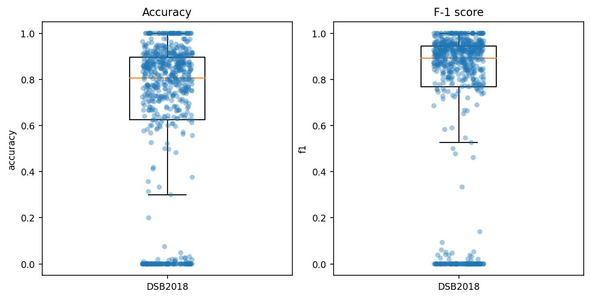
It performs pretty well overall!
Scaling up evaluation#
We saw that iterating DSB2018 dataset can be easily done with bioimageloader. Likewise, it is simple to iterate all other datasets in the same steps.
Below, I am loading datasets that have instance segmented mask annotation, so that I can get object detection related metrics in the end. In addition, I am converting color images to grayscale with grayscale argument, because StarDist expects that.
NOTE that we are using training dataset for DSB2018 and BBBC039 (the others do not have splits). Take this fact into account when you analyze results below.
[15]:
cfg_all_collections = Config('../configs/instance_mask_collections_gray.yml')
cfg_all_collections
[15]:
{'DSB2018': {'root_dir': '/home/seongbinlim/Data/DSB2018/', 'grayscale': True},
 'ComputationalPathology': {'root_dir': '/home/seongbinlim/Data/ComputationalPathology',
  'grayscale': True},
 'S_BSST265': {'root_dir': '/home/seongbinlim/Data/BioStudies'},
 'FRUNet': {'root_dir': '/home/seongbinlim/Data/FRU_processing'},
 'BBBC006': {'root_dir': '/home/seongbinlim/Data/bbbc/006/',
  'grayscale': True},
 'BBBC020': {'root_dir': '/home/seongbinlim/Data/bbbc/020', 'grayscale': True},
 'BBBC039': {'root_dir': '/home/seongbinlim/Data/bbbc/039'}}
[16]:
transforms = A.Compose([
    A.Resize(256, 256),
    SqueezeGrayImageHWC()  # from (h, w, 3) to (h, w)
])
[17]:
datasets = cfg_all_collections.load_datasets(transforms=transforms)
total_len = 0
for dset in datasets:
    total_len += len(dset)
    print(f'{dset.acronym:10s}: {len(dset):10d}')
print('{:10s}: {:10d}'.format('total', total_len))
DSB2018   :        670
ComPath   :         30
S_BSST265 :         79
FRUNet    :         72
BBBC006   :        768
BBBC020   :         20
BBBC039   :        150
total     :       1789
[18]:
BATCH_SIZE = 32
NUM_WORKERS = 8

scores_df = pd.DataFrame(columns=['Name', 'Accuracy', 'F-1'])
for dset in datasets:
    print('Iterating:', dset.acronym)
    loader = BatchDataloader(dset,
                             batch_size=BATCH_SIZE,
                             num_workers=NUM_WORKERS)
    iter_loader = iter(loader)
    for batch in tqdm(iter_loader, total=len(loader)):
        input_image = batch['image']
        gt_mask = batch['mask']
        # will have shape (BATCH_SIZE, 256, 256)
        b = len(input_image)

        for i in range(b):
            input_image_i = normalize(input_image[i])
            gt_mask_i = gt_mask[i]
            pred_i, _ = model.predict_instances(input_image_i)
            score = matching(gt_mask_i, pred_i)
            scores_df.loc[len(scores_df)] = dset.acronym, score.accuracy, score.f1
Iterating: DSB2018
Iterating: ComPath
Iterating: S_BSST265
Iterating: FRUNet
Iterating: BBBC006
Iterating: BBBC020
Iterating: BBBC039
Do some pandas juggling. Make each column represent a dataset and get Accuracy.
[19]:
pivot_scores_acc = scores_df.pivot(columns='Name', values='Accuracy')
pivot_scores_acc
[19]:
| Name | BBBC006 | BBBC020 | BBBC039 | ComPath | DSB2018 | FRUNet | S_BSST265 |
|---|---|---|---|---|---|---|---|
| 0 | NaN | NaN | NaN | NaN | 0.740741 | NaN | NaN |
| 1 | NaN | NaN | NaN | NaN | 0.944444 | NaN | NaN |
| 2 | NaN | NaN | NaN | NaN | 0.000000 | NaN | NaN |
| 3 | NaN | NaN | NaN | NaN | 0.000000 | NaN | NaN |
| 4 | NaN | NaN | NaN | NaN | 0.000000 | NaN | NaN |
| ... | ... | ... | ... | ... | ... | ... | ... |
| 1784 | NaN | NaN | 0.875000 | NaN | NaN | NaN | NaN |
| 1785 | NaN | NaN | 0.778626 | NaN | NaN | NaN | NaN |
| 1786 | NaN | NaN | 0.909091 | NaN | NaN | NaN | NaN |
| 1787 | NaN | NaN | 0.876190 | NaN | NaN | NaN | NaN |
| 1788 | NaN | NaN | 0.896226 | NaN | NaN | NaN | NaN |
1789 rows × 7 columns
Remove NaN and serialize each column individually
[20]:
scores_acc = []
for dset in datasets:
    scores_acc.append(pivot_scores_acc[dset.acronym].dropna().reset_index(drop=True))
[21]:
# props
medianprops = dict(color='k', alpha=0.5)
boxprops = dict(linestyle='-', linewidth=1)
meanpointprops = dict(marker='*',
markersize=5,
markerfacecolor='k',
markeredgecolor='none',
)
pos = list(range(len(pivot_scores_acc.columns))) # sns default
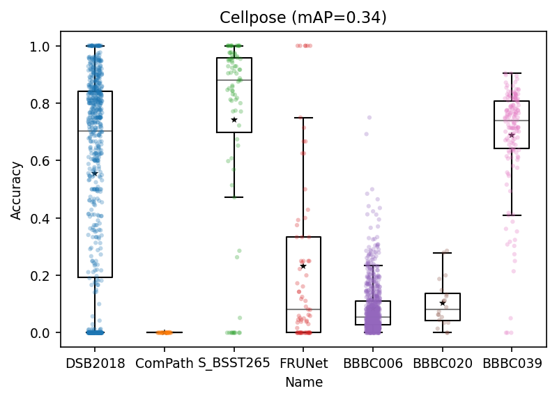
mAP = scores_df.Accuracy.mean()
fig, ax = plt.subplots(dpi=150)
ax.boxplot(scores_acc,
positions=pos,
meanline=False,
showmeans=True,
showfliers=False,
boxprops=boxprops,
medianprops=medianprops,
meanprops=meanpointprops,
)
sns.stripplot(x='Name', y='Accuracy', data=scores_df,
size=3, alpha=0.3, ax=ax)
# ax.set_ylim(bottom=0.4)
ax.set_title(f'StarDist (mAP={mAP:.2f})')
[21]:
Text(0.5, 1.0, 'StarDist (mAP=0.50)')
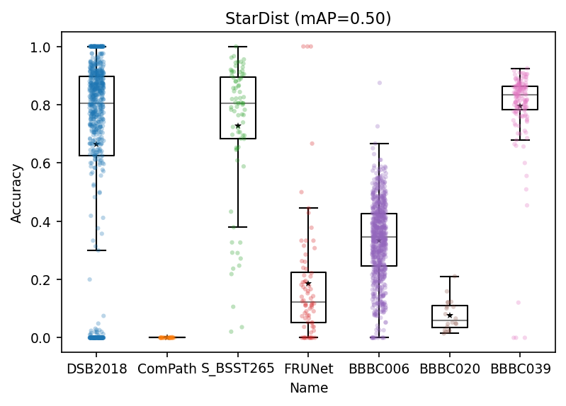
Overall StarDist is very impressive!
[Some More] Accuracy (average precision) value of ComPath is brutal. Did we do something wrong? Check out the last section in this notebook 1.4. [Some More] Fixing(?) ComPath if you are interested.
Cellpose#
Test Cellpose#
[22]:
model_cp = cellpose_models.Cellpose(
    gpu=True if torch.cuda.is_available() else False,
    model_type='nuclei',
)
[23]:
img = test_image_nuclei_2d()

with torch.no_grad():
    mask, _, _, _ = model_cp.eval(img)
[24]:
fig, ax = plt.subplots(ncols=2, dpi=150)
ax[0].imshow(img)
ax[1].imshow(mask, cmap=cmap)
[24]:
<matplotlib.image.AxesImage at 0x7fe9c9c24520>
Evaluation with Cellpose and bioimageloader#
Below code cells are almost copy-paste form StarDist parts except for some parts.
[25]:
cfg_all_collections
[25]:
{'DSB2018': {'root_dir': '/home/seongbinlim/Data/DSB2018/', 'grayscale': True},
 'ComputationalPathology': {'root_dir': '/home/seongbinlim/Data/ComputationalPathology',
  'grayscale': True},
 'S_BSST265': {'root_dir': '/home/seongbinlim/Data/BioStudies'},
 'FRUNet': {'root_dir': '/home/seongbinlim/Data/FRU_processing'},
 'BBBC006': {'root_dir': '/home/seongbinlim/Data/bbbc/006/',
  'grayscale': True},
 'BBBC020': {'root_dir': '/home/seongbinlim/Data/bbbc/020', 'grayscale': True},
 'BBBC039': {'root_dir': '/home/seongbinlim/Data/bbbc/039'}}
Cellpose expect image batch to have (b, 3, h, w) shape. Remember that bioimageloader returns (b, h, w, 3)? We will reorder shape to match what Cellpose requires by using bioimageloader.transforms.HWCToCHW.
[26]:
transforms = A.Compose([
    A.Resize(256, 256),
    # SqueezeGrayImageHWC()  # from (h, w, 3) to (h, w)
    HWCToCHW(),  # NEW, from (h, w, 3) to (3, h, w)
])
[27]:
datasets = cfg_all_collections.load_datasets(transforms=transforms)
total_len = 0
for dset in datasets:
    total_len += len(dset)
    print(f'{dset.acronym:10s}: {len(dset):10d}')
print('{:10s}: {:10d}'.format('total', total_len))
DSB2018   :        670
ComPath   :         30
S_BSST265 :         79
FRUNet    :         72
BBBC006   :        768
BBBC020   :         20
BBBC039   :        150
total     :       1789
We will go through the same steps as StarDist
Notice that
Cellpose allows batch processing
Don’t have to iterate each entry in batch
Slower than StarDist because of
net_avgYou may think that batch processing should allow faster execution, but it is not because of
net_avg. It is an ensemble idea, common in machine learning. Cellpose suggests to opt innet_avg, which runs 4 differenct models and aggregates their results.
[28]:
BATCH_SIZE = 32
NUM_WORKERS = 8

scores_df = pd.DataFrame(columns=['Name', 'Accuracy', 'F-1'])
for dset in datasets:
    print('Iterating:', dset.acronym)
    loader = BatchDataloader(dset,
                             batch_size=BATCH_SIZE,
                             num_workers=NUM_WORKERS)
    iter_loader = iter(loader)
    for batch in tqdm(iter_loader, total=len(loader)):
        input_image = batch['image']
        gt_mask = batch['mask']
        # will have shape (BATCH_SIZE, 256, 256)
        b = len(input_image)
        with torch.no_grad():
            pred_mask, _, _, _ = model_cp.eval(input_image,
                                               normalize=True,
                                               net_avg=True)
        for i in range(b):
            gt_mask_i = gt_mask[i]
            pred_i = pred_mask[i]
            score = matching(gt_mask_i, pred_i)
            scores_df.loc[len(scores_df)] = dset.acronym, score.accuracy, score.f1
Iterating: DSB2018
WARNING: no mask pixels found
Iterating: ComPath
Iterating: S_BSST265
Iterating: FRUNet
WARNING: no mask pixels found
Iterating: BBBC006
Iterating: BBBC020
Iterating: BBBC039
[29]:
scores_df
[29]:
| Name | Accuracy | F-1 | |
|---|---|---|---|
| 0 | DSB2018 | 0.714286 | 0.833333 |
| 1 | DSB2018 | 0.861111 | 0.925373 |
| 2 | DSB2018 | 0.000000 | 0.000000 |
| 3 | DSB2018 | 0.000000 | 0.000000 |
| 4 | DSB2018 | 0.000000 | 0.000000 |
| ... | ... | ... | ... |
| 1784 | BBBC039 | 0.791667 | 0.883721 |
| 1785 | BBBC039 | 0.732824 | 0.845815 |
| 1786 | BBBC039 | 0.830769 | 0.907563 |
| 1787 | BBBC039 | 0.764151 | 0.866310 |
| 1788 | BBBC039 | 0.828571 | 0.906250 |
1789 rows × 3 columns
[30]:
pivot_scores_acc = scores_df.pivot(columns='Name', values='Accuracy')
pivot_scores_acc
[30]:
| Name | BBBC006 | BBBC020 | BBBC039 | ComPath | DSB2018 | FRUNet | S_BSST265 |
|---|---|---|---|---|---|---|---|
| 0 | NaN | NaN | NaN | NaN | 0.714286 | NaN | NaN |
| 1 | NaN | NaN | NaN | NaN | 0.861111 | NaN | NaN |
| 2 | NaN | NaN | NaN | NaN | 0.000000 | NaN | NaN |
| 3 | NaN | NaN | NaN | NaN | 0.000000 | NaN | NaN |
| 4 | NaN | NaN | NaN | NaN | 0.000000 | NaN | NaN |
| ... | ... | ... | ... | ... | ... | ... | ... |
| 1784 | NaN | NaN | 0.791667 | NaN | NaN | NaN | NaN |
| 1785 | NaN | NaN | 0.732824 | NaN | NaN | NaN | NaN |
| 1786 | NaN | NaN | 0.830769 | NaN | NaN | NaN | NaN |
| 1787 | NaN | NaN | 0.764151 | NaN | NaN | NaN | NaN |
| 1788 | NaN | NaN | 0.828571 | NaN | NaN | NaN | NaN |
1789 rows × 7 columns
Remove NaN and serialize each column individually
[31]:
scores_acc = []
for dset in datasets:
    scores_acc.append(pivot_scores_acc[dset.acronym].dropna().reset_index(drop=True))
[32]:
# props
medianprops = dict(color='k', alpha=0.5)
boxprops = dict(linestyle='-', linewidth=1)
meanpointprops = dict(marker='*',
                      markersize=5,
                      markerfacecolor='k',
                      markeredgecolor='none',
                     )


pos = list(range(len(pivot_scores_acc.columns)))  # sns default
mAP = scores_df.Accuracy.mean()

fig, ax = plt.subplots(dpi=150)
ax.boxplot(scores_acc,
           positions=pos,
           meanline=False,
           showmeans=True,
           showfliers=False,
           boxprops=boxprops,
           medianprops=medianprops,
           meanprops=meanpointprops,
          )
sns.stripplot(x='Name', y='Accuracy', data=scores_df,
              size=3, alpha=0.3, ax=ax)
# ax.set_ylim(bottom=0.4)
ax.set_title(f'Cellpose (mAP={mAP:.2f})')
[32]:
Text(0.5, 1.0, 'Cellpose (mAP=0.34)')
Again as I mentioned at the beginning of this notbook, there is no winner! Cellpose does better in some cases and does not in others. Depending on your images and tasks, you decide which to use, what pre-/post-processes are needed on top of that, how to normalize your data so that they get fit to these models, etc.
You definitely want to analyze and get statistics of your data before you do anything on them, and now you have bioimageloader that could make all these steps so much easier and much painless!
[Some More] Fixing(?) ComPath#
This overview table is a helpful one. You could see from the sample images that ComPath is, first of all, H&E histopathology images, which are distinct from the others. And images are dense and have high resolution (1000, 1000). So resizing them to (256, 256) may have not been a wise choice for ComPath.
Let’s define a new set of transforms for ComPath. We are going to do two things:
Remove
Resize()so that StarDist processes large dense images of ComPathStarDist is a family of FCN (Fully Connected Neural network), which has size-invariant property meaning that it can take any size of input and return ouput whose size is the same as that of input. So we can just get rid of Resize.
albumentation.InvertImg(p=1.0)It will invert pixel values with 100% probability (
p=1.0). It will make H&E stained images look more like the rest.
[33]:
cfg_all_collections
[33]:
{'DSB2018': {'root_dir': '/home/seongbinlim/Data/DSB2018/', 'grayscale': True},
 'ComputationalPathology': {'root_dir': '/home/seongbinlim/Data/ComputationalPathology',
  'grayscale': True},
 'S_BSST265': {'root_dir': '/home/seongbinlim/Data/BioStudies'},
 'FRUNet': {'root_dir': '/home/seongbinlim/Data/FRU_processing'},
 'BBBC006': {'root_dir': '/home/seongbinlim/Data/bbbc/006/',
  'grayscale': True},
 'BBBC020': {'root_dir': '/home/seongbinlim/Data/bbbc/020', 'grayscale': True},
 'BBBC039': {'root_dir': '/home/seongbinlim/Data/bbbc/039'}}
[34]:
transforms = A.Compose([
    A.Resize(256, 256),
    SqueezeGrayImageHWC()  # from (h, w, 3) to (h, w)
])
transforms_compath = A.Compose([
    A.InvertImg(p=1.0),
    SqueezeGrayImageHWC()  # from (h, w, 3) to (h, w)
])

cfg_transforms = {
    'DSB2018': transforms,
    'ComputationalPathology': transforms_compath,  # needs extra care
    'S_BSST265': transforms,
    'FRUNet': transforms,
    'BBBC006': transforms,
    'BBBC020': transforms,
    'BBBC039': transforms,
}
[35]:
# we only need ComPath
datasets = cfg_all_collections.load_datasets(transforms=cfg_transforms)
dset = datasets[1]
print(dset)
ComPath
[36]:
BATCH_SIZE = 32
NUM_WORKERS = 8

fix_scores_df = pd.DataFrame(columns=['Name', 'Accuracy', 'F-1'])
# for dset in datasets:
print(dset.acronym)
loader = BatchDataloader(dset,
                         batch_size=BATCH_SIZE,
                         num_workers=NUM_WORKERS)
iter_loader = iter(loader)
for batch in tqdm(iter_loader, total=len(loader)):
    input_image = batch['image']
    gt_mask = batch['mask']
    # will have shape (BATCH_SIZE, 256, 256)
    b = len(input_image)

    for i in range(b):
        input_image_i = normalize(input_image[i])
        gt_mask_i = gt_mask[i]
        pred_i, _ = model.predict_instances(input_image_i)
        score = matching(gt_mask_i, pred_i)
        fix_scores_df.loc[len(fix_scores_df)] = dset.acronym, score.accuracy, score.f1
ComPath
[37]:
beforefix_scores = pivot_scores_acc['ComPath'].dropna().reset_index(drop=True)
beforefix_scores.head()
# before, almost all values were close to zero
[37]:
0    0.0
1    0.0
2    0.0
3    0.0
4    0.0
Name: ComPath, dtype: float64
[38]:
fix_scores_df.head()
# new metrics look much better. they are not zeros!
[38]:
| Name | Accuracy | F-1 | |
|---|---|---|---|
| 0 | ComPath | 0.382353 | 0.553191 |
| 1 | ComPath | 0.394756 | 0.566057 |
| 2 | ComPath | 0.348028 | 0.516351 |
| 3 | ComPath | 0.133023 | 0.234811 |
| 4 | ComPath | 0.093212 | 0.170528 |
[39]:
# props
medianprops = dict(color='k', alpha=0.5)
boxprops = dict(linestyle='-', linewidth=1)
meanpointprops = dict(marker='*',
                      markersize=5,
                      markerfacecolor='k',
                      markeredgecolor='none',
                     )


pos = [0]  # sns default
# mAP = scores_df.Accuracy.mean()

fig, ax = plt.subplots(ncols=2, sharey=True, dpi=150)
ax[0].boxplot(beforefix_scores,
           positions=pos,
           meanline=False,
           showmeans=True,
           showfliers=False,
           boxprops=boxprops,
           medianprops=medianprops,
           meanprops=meanpointprops,
          )
sns.stripplot(y=beforefix_scores,
              size=3, alpha=0.3, ax=ax[0])
ax[0].set_ylabel('Accuracy')
ax[0].set_xticklabels(['Before Fix'])

ax[1].boxplot(fix_scores_df.Accuracy,
           positions=pos,
           meanline=False,
           showmeans=True,
           showfliers=False,
           boxprops=boxprops,
           medianprops=medianprops,
           meanprops=meanpointprops,
          )
sns.stripplot(x='Name', y='Accuracy', data=fix_scores_df,
              size=3, alpha=0.3, ax=ax[1])
ax[1].set_xticklabels(['After Fix'])
ax[1].set_xlabel('')
fig.suptitle('ComPath')
[39]:
Text(0.5, 0.98, 'ComPath')
We can visualize actual predictions
[40]:
# sample first two paris
for ind in range(2):
    data = dset[ind]
    image = data['image']
    mask = data['mask']
    pred, _ = model.predict_instances(normalize(image))
    score = matching(mask, pred)

    with plt.rc_context({'image.interpolation': 'none'}):
        fig, ax = plt.subplots(ncols=3, figsize=[10, 4], dpi=150)
        fig.suptitle(f'ComPath({ind+1}/{len(dset)}) (accuracy: {score.accuracy:.2f})')
        ax[0].imshow(image)
        ax[0].set_title('Input image')
        ax[1].imshow(mask, cmap=cmap)
        ax[1].set_title('Ground truth')
        ax[2].imshow(pred, cmap=cmap)
        ax[2].set_title('StarDist prediction')
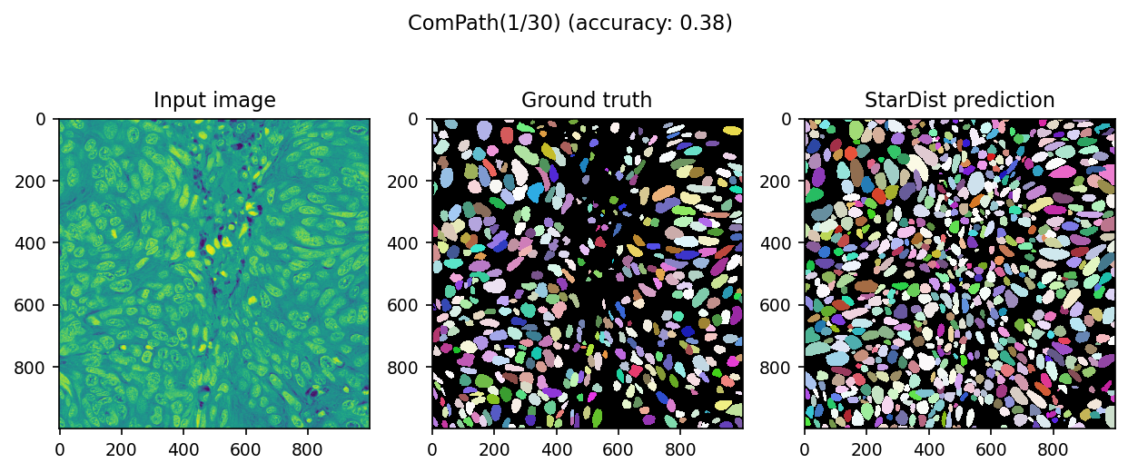
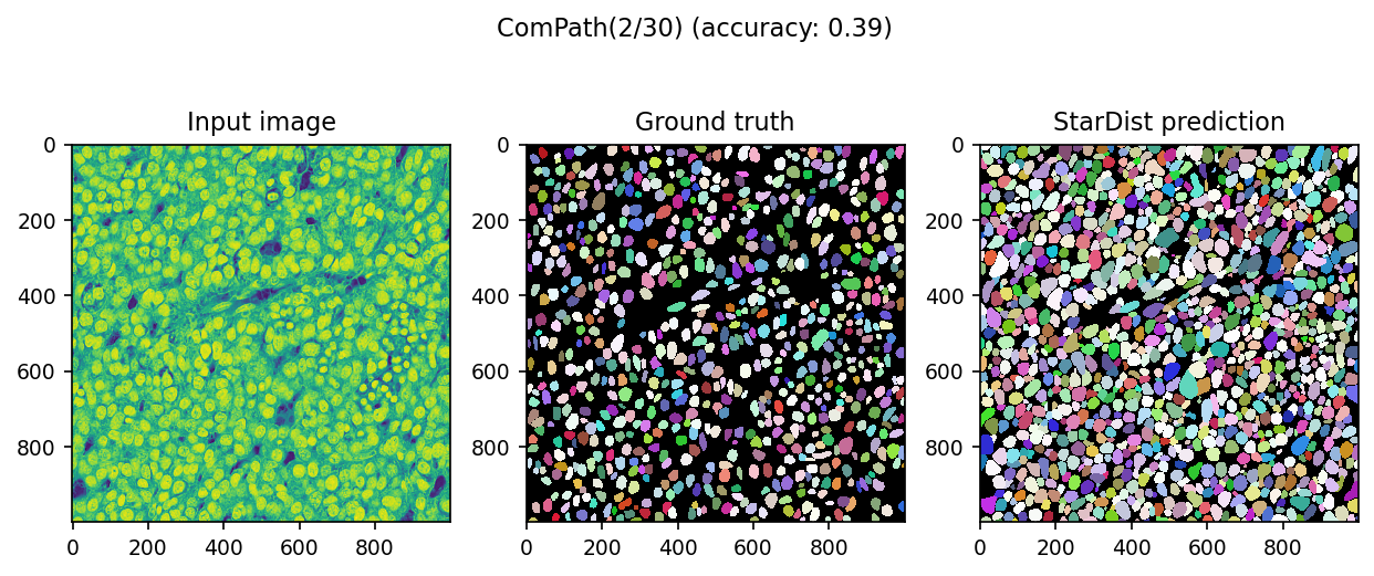
We fixed(?) it from almost zero prediction!