DL: Benchmark Table#

Date: 2022-05-05
Author: Xingjian Zhang (https://github.com/xjzhaang)

In this notebook, we build a benchmark table using the built-in models from StarDist and Cellpose as well as our trained models from the previous notebook DL: Training Stardist and Cellpose Models.

The first section shows how to obtain the predictions from our custom trained models. The second section includes the code for building the table, using seaborn and matplotlib.

Evaluate a custom model#

1. StarDist#

In this section, we show how to get predictions from the StarDist model that we had trained.

Many of it is similar to the contents of DL: StarDist and Cellpose. You can skip to the next section to find the code for building the benchmark table.

[1]:

%env CUDA_VISIBLE_DEVICES=0
%env TF_CPP_MIN_LOG_LEVEL=3

#Built-in
import warnings
import logging
import sys
from pathlib import Path

#Ignoring warnings for notebook compilation
warnings.filterwarnings('ignore')
logging.getLogger("tensorflow").setLevel(logging.ERROR)

#Bioimageloader and Albumentation
import albumentations as A
from bioimageloader import Config, BatchDataloader
from bioimageloader.transforms import SqueezeGrayImageHWC, HWCToCHW

#Stardist and Tensorflow
import tensorflow as tf
from stardist.matching import matching, matching_dataset
from stardist.models import StarDist2D

#Cellpose and Torch
import torch
from cellpose import models as cellpose_models

#Other imports
#!pip install matplotlib seaborn pandas tqdm numpy
import pandas as pd
import glob
import numpy as np
import matplotlib.pyplot as plt
import seaborn as sns

env: CUDA_VISIBLE_DEVICES=0
env: TF_CPP_MIN_LOG_LEVEL=3

[2]:

# setting 'TF_FORCE_GPU_ALLOW_GROWTH' does not actually limit
# gpu memory, it allows to grow. we have to manually limit memory usage
if gpus := tf.config.list_physical_devices('GPU'):
    for gpu in gpus:
        try:
            vdc = tf.config.experimental.VirtualDeviceConfiguration(
                memory_limit=2000
            )
            tf.config.experimental.set_virtual_device_configuration(
                gpu, [vdc]
            )
        except RuntimeError as e:
            print(e)
# see what devices you have (set)
print(tf.config.list_physical_devices())

[PhysicalDevice(name='/physical_device:CPU:0', device_type='CPU'), PhysicalDevice(name='/physical_device:GPU:0', device_type='GPU')]

We load the datasets together using a config file and apply transformations. We invert ComPath and LIVECell as we had trained our model with them inverted.

[3]:

cfg_all_collections = Config('configs/instanceseg.yml')
transforms = A.Compose([
    A.Resize(256, 256),
    SqueezeGrayImageHWC()
])
transforms_invert = A.Compose([
    A.InvertImg(p=1.0),
    SqueezeGrayImageHWC()
])

cfg_transforms = {
    'DSB2018': transforms,
    'ComputationalPathology': transforms_invert,
    'S_BSST265': transforms,
    'FRUNet': transforms,
    'BBBC006': transforms,
    'BBBC020': transforms,
    'BBBC039': transforms,
    'Cellpose': transforms,
    'LIVECell': transforms_invert,
}
datasets = cfg_all_collections.load_datasets(transforms=cfg_transforms)
total_len = 0
for dset in datasets:
    total_len += len(dset)
    print(f'{dset.acronym:10s}: {len(dset):10d}')
print('{:10s}: {:10d}'.format('total', total_len))

DSB2018   :        670
ComPath   :         30
S_BSST265 :         79
FRUNet    :         72
BBBC006   :        768
BBBC020   :         20
BBBC039   :        150
Cellpose  :        540
LIVECell  :       1512
total     :       3841

Loading the custom model#

We load the trained model by specifying its name and base directory.

[4]:

name='stardist_model_1'  #name of the model folder
basedir='stardist_models'  #base directory the model folder is in
model_sd = StarDist2D(None, name=name,basedir=basedir)

Loading network weights from 'weights_best.h5'.
Loading thresholds from 'thresholds.json'.
Using default values: prob_thresh=0.198454, nms_thresh=0.3.

Evaluation#

We predict the F-1 and Average Precision (by definition of DSB2018 challenge). The scores are saved in a csv file in a folder ./csvs

[ ]:

BATCH_SIZE = 64
NUM_WORKERS = 12

scores_df = pd.DataFrame(columns=['Name', 'Accuracy', 'F-1'])
for dset in datasets:
    conf_iou_list = []
    diff = 0
    check = 0
    print('Iterating:', dset.acronym)
    loader = BatchDataloader(dset,
                             batch_size=BATCH_SIZE,
                             num_workers=NUM_WORKERS)
    iter_loader = iter(loader)

    for batch in tqdm(iter_loader, total=len(loader)):
        input_image = batch['image']
        gt_mask = batch['mask']
        # will have shape (BATCH_SIZE, 256, 256)
        b = len(input_image)
        for i in range(b):
            input_image_i = normalize(input_image[i])
            gt_mask_i = gt_mask[i]
            pred_i, _ = model_sd.predict_instances(input_image_i)
            score = matching(gt_mask_i, pred_i)
            scores_df.loc[len(scores_df)] = dset.acronym, score.accuracy, score.f1

#Save the score dataframe to a csv. We will load these csv to build our benchmark table
scores_df.to_csv('csvs/trained_stardist.csv')

2. Cellpose#

For the custom cellpose model, the procedure is similar except we use HWCToCHW instead.

[5]:

cfg_all_collections = Config('configs/instanceseg.yml')
transforms = A.Compose([
    A.Resize(256, 256),
    HWCToCHW()
])
transforms_invert = A.Compose([
    A.InvertImg(p=1.0),
    HWCToCHW()
])

cfg_transforms = {
    'DSB2018': transforms,
    'ComputationalPathology': transforms_invert,
    'S_BSST265': transforms,
    'FRUNet': transforms,
    'BBBC006': transforms,
    'BBBC020': transforms,
    'BBBC039': transforms,
    'Cellpose': transforms,
    'LIVECell': transforms_invert,
}
datasets = cfg_all_collections.load_datasets(transforms=cfg_transforms)
total_len = 0
for dset in datasets:
    total_len += len(dset)
    print(f'{dset.acronym:10s}: {len(dset):10d}')
print('{:10s}: {:10d}'.format('total', total_len))

DSB2018   :        670
ComPath   :         30
S_BSST265 :         79
FRUNet    :         72
BBBC006   :        768
BBBC020   :         20
BBBC039   :        150
Cellpose  :        540
LIVECell  :       1512
total     :       3841

Loading the custom model#

We load the cellpose trained model by specifying its entire path as pretrained_model.

[6]:

pretrained_model = "cellpose_models/cellpose_model_1"
model_cp = cellpose_models.CellposeModel(
    gpu=True if torch.cuda.is_available() else False,
    pretrained_model = pretrained_model,
)

Evaluation#

[ ]:

BATCH_SIZE = 64
NUM_WORKERS = 12

scores_df = pd.DataFrame(columns=['Name', 'Accuracy', 'F-1'])
for dset in datasets:
    print('Iterating:', dset.acronym)
    loader = BatchDataloader(dset,
                             batch_size=BATCH_SIZE,
                             num_workers=NUM_WORKERS)
    iter_loader = iter(loader)
    for batch in tqdm(iter_loader, total=len(loader)):
        input_image = batch['image']
        gt_mask = batch['mask']

        # will have shape (BATCH_SIZE, 256, 256)
        b = len(input_image)

        with torch.no_grad():
            pred_mask, _, _ = model_cp.eval(input_image, channels = [0,0],
                                            normalize=True,
                                            net_avg=True)
        for i in range(b):
            gt_mask_i = gt_mask[i]
            pred_i = pred_mask[i]
            score = matching(gt_mask_i, pred_i)
            scores_df.loc[len(scores_df)] = dset.acronym, score.accuracy, score.f1

#Save the score dataframe to a csv. We will load these csv to build our benchmark table
scores_df.to_csv('csvs/trained_cellpose.csv')

Build a Benchmark Table#

In this section, we will use the csv files to build a benchmark table.

Note: This notebook does not include the code for predicting the built-in models. To have all the csv files, you need to run those models.

[7]:

# Intiate the table heads by reading one of the csvs
headers = pd.read_csv("csvs/trained_stardist.csv")
table_f1 = pd.DataFrame({'Name': headers.Name.unique(),})
table_ap = pd.DataFrame({'Name': headers.Name.unique(),})

[8]:

# Iterate through the ./csvs folder and build a table
path = "csvs/*.csv"
for fname in glob.glob(path):
    data = pd.read_csv(fname)
    grouped = data.groupby(data.Name)
    model_name = Path(fname).stem
    table_f1[model_name] = ""
    table_ap[model_name] = ""
    for name, group in grouped:
        table_f1[model_name][table_f1.Name == name] = float(group["F-1"].mean())
        table_ap[model_name][table_ap.Name == name] = float(group["Accuracy"].mean())

[9]:

table =  pd.concat([table_f1, table_ap], keys=('F-1 score','AP score (DSB2018 def.)'))
table

[9]:

		Name	cellpose_cyto	cellpose_livecell	cellpose_cyto2	stardist_2D_versatile_fluo	cellpose_tissuenet	stardist_2D_paper_dsb2018	cellpose_nuclei	trained_stardist	trained_cellpose
F-1 score	0	DSB2018	0.730809	0.229489	0.640016	0.723228	0.08416	0.734636	0.679816	0.771526	0.822517
	1	ComPath	0.605584	0.019909	0.619825	0.397856	0.002566	0.014182	0.848293	0.451944	0.73797
	2	S_BSST265	0.771823	0.324273	0.785657	0.812577	0.169406	0.82551	0.788799	0.866933	0.82654
	3	FRUNet	0.334177	0.040874	0.383345	0.271294	0.001389	0.246895	0.337578	0.586409	0.425578
	4	BBBC006	0.901021	0.000573	0.881132	0.899666	0.0002	0.896641	0.866544	0.900995	0.906193
	5	BBBC020	0.208807	0.002273	0.334287	0.688047	0.002941	0.721832	0.832275	0.655209	0.901965
	6	BBBC039	0.863331	0.391755	0.833369	0.874683	0.0	0.889251	0.907173	0.877522	0.912593
	7	Cellpose	0.71751	0.173615	0.725331	0.285131	0.083296	0.301175	0.216199	0.55468	0.67811
	8	LIVECell	0.077161	0.762824	0.036689	0.003265	0.0	0.022424	0.017852	0.471298	0.668026
AP score (DSB2018 def.)	0	DSB2018	0.629021	0.150537	0.533594	0.66345	0.055726	0.684467	0.616813	0.675894	0.745665
	1	ComPath	0.452814	0.010872	0.465145	0.261882	0.001306	0.007352	0.741976	0.306428	0.59969
	2	S_BSST265	0.717085	0.215294	0.741428	0.726089	0.10996	0.749204	0.722878	0.789683	0.769494
	3	FRUNet	0.275127	0.028123	0.32523	0.185416	0.000731	0.159862	0.247326	0.468514	0.324919
	4	BBBC006	0.835181	0.000296	0.809011	0.829919	0.000109	0.825314	0.78227	0.833109	0.843333
	5	BBBC020	0.137004	0.001163	0.238752	0.570059	0.001515	0.588421	0.718742	0.540832	0.825222
	6	BBBC039	0.781059	0.25284	0.738465	0.795909	0.0	0.819462	0.853814	0.799828	0.860373
	7	Cellpose	0.62084	0.121824	0.630782	0.20269	0.059715	0.211034	0.146796	0.415835	0.560193
	8	LIVECell	0.043625	0.641513	0.020076	0.001678	0.0	0.011679	0.009352	0.335946	0.528168

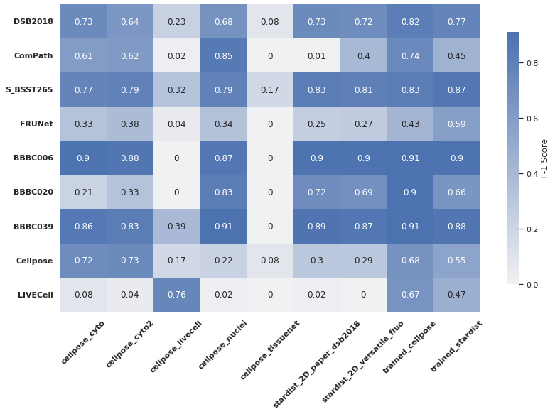
Heat map for F-1 scores#

Let us build a heat map using the F-1 scores. The scores were saved in the dataframe table_f1

[10]:

#Some table juggling
heat_f1 = table_f1.reindex(sorted(table_f1.columns), axis=1)
s = table_f1.select_dtypes(include='object').columns[1:]
heat_f1[s] = heat_f1[s].astype("float")

heat = heat_f1.round(2).to_numpy()
heat = [heat[i, 1:] for i in range(len(heat))]
heat = np.array(heat).astype("float64")

Here is the plot.

[11]:

sns.set_theme(style="ticks", color_codes=True)
coolwarm = sns.color_palette("coolwarm_r", as_cmap=True)
mono = sns.color_palette("light:b", as_cmap=True)
sns.set(rc={'figure.figsize':(11.7,8.27)})
plot = sns.heatmap(heat,
                   cmap=mono,
                   xticklabels=heat_f1.columns.drop("Name"),
                   yticklabels=table_f1.Name,
                   annot=True,
                   cbar_kws={'label': 'F-1 Score', "shrink": .82,})
plot.set_xticklabels(plot.get_xticklabels(),rotation=45, fontweight = 'bold')
plot.set_yticklabels(plot.get_yticklabels(), fontweight = 'bold')
plt.tight_layout()
plt.show()